posting rubric and sample code
jekyll and knitr examples from http://yihui.name/knitr-jekyll/2014/09/jekyll-with-knitr.html
The R package servr can be used to set up an HTTP server to serve files under a directory. Since servr v0.2, it has added a function servr::jekyll() specifically designed for websites based on Jekyll and R Markdown. The main features of this function are:
- R Markdown source files are re-compiled through knitr when their corresponding Markdown output files become older1 than source files;
- The web page will refresh itself automatically in the above case as well;
As a result, all you need to do is write your blog posts (R Markdown documents), and you do not need to worry about re-building the website or calling knitr commands. Whenever you save a blog post in your text editor, the web page will be updated on the fly. This is particularly handy in the RStudio IDE, because after you run servr::jekyll() in the console, you can start writing or editing your R Markdown posts, and the HTML output, displayed in the RStudio viewer pane, will be in sync with your source post in the source panel (see the screenshot below).

Prerequisites
You must have installed the packages servr (>= 0.2) and knitr (>= 1.8).
install.packages(c("servr", "knitr"), repos = "http://cran.rstudio.com")Of course, you have to install Jekyll as well. For Windows users, you have to make sure jekyll can be found from your environment variable PATH, i.e., R can call it via system('jekyll'). This is normally not an issue for Linux or Mac OS X users (gem install jekyll is enough).
R code chunks
Now we write some R code chunks in this post. For example,
options(digits = 3)
cat("hello world!")
## hello world!set.seed(123)
(x = rnorm(40) + 10)## [1] 9.44 9.77 11.56 10.07 10.13 11.72 10.46 8.73 9.31 9.55 11.22
## [12] 10.36 10.40 10.11 9.44 11.79 10.50 8.03 10.70 9.53 8.93 9.78
## [23] 8.97 9.27 9.37 8.31 10.84 10.15 8.86 11.25 10.43 9.70 10.90
## [34] 10.88 10.82 10.69 10.55 9.94 9.69 9.62# generate a table
knitr::kable(head(mtcars))| mpg | cyl | disp | hp | drat | wt | qsec | vs | am | gear | carb | |
|---|---|---|---|---|---|---|---|---|---|---|---|
| Mazda RX4 | 21.0 | 6 | 160 | 110 | 3.90 | 2.62 | 16.5 | 0 | 1 | 4 | 4 |
| Mazda RX4 Wag | 21.0 | 6 | 160 | 110 | 3.90 | 2.88 | 17.0 | 0 | 1 | 4 | 4 |
| Datsun 710 | 22.8 | 4 | 108 | 93 | 3.85 | 2.32 | 18.6 | 1 | 1 | 4 | 1 |
| Hornet 4 Drive | 21.4 | 6 | 258 | 110 | 3.08 | 3.21 | 19.4 | 1 | 0 | 3 | 1 |
| Hornet Sportabout | 18.7 | 8 | 360 | 175 | 3.15 | 3.44 | 17.0 | 0 | 0 | 3 | 2 |
| Valiant | 18.1 | 6 | 225 | 105 | 2.76 | 3.46 | 20.2 | 1 | 0 | 3 | 1 |
(function() {
    if (TRUE)
        1 + 1  # a boring comment
})()
## [1] 2names(formals(servr::jekyll)) # arguments of the jekyll() function## [1] "dir" "input" "output" "script" "serve" "command"
## [7] "..."Just to test inline R expressions2 in knitr, we know the first element in x (created in the code chunk above) is 9.44. You can certainly draw some graphs as well:
par(mar = c(4, 4, 0.1, 0.1))
plot(cars, pch = 19, col = "red")  # a scatterplot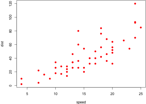
The build script
Zero-configuration is required for servr::jekyll() to work on your Jekyll website. However, there is always demand for more control over some options, which can be defined in a custom build script. Here are the arguments of servr::jekyll():
jekyll(dir = ".", input = c(".", "_source", "_posts"), output = c(".",
    "_posts", "_posts"), script = c("Makefile", "build.R"), serve = TRUE,
    command = "jekyll build", ...)
By default, jekyll() looks for .Rmd files under the root directory, the _source directory, and the _posts directory of the Jekyll website. For example, if you put your R Markdown posts under _source, they will be compiled to the _posts directory3.
The script argument specifies a Makefile or an R script to be used to compile your R Markdown files. If it is a Makefile, jekyll() will run make -q to see if the site needs to be recompiled, then make if it does. If the script is an R script, say, named build.R, it is called via command line of the form
Rscript build.R arg1 arg2
See ?servr::jekyll for more details. You can define all your knitr options and any other options in this R script. See the script build.R in the knitr-jekyll repository for an example: it will automatically set up the output renderers for knitr, e.g., when the Jekyll Markdown engine is kramdown, this script will call knitr::render_jekyll() so that the code chunk output will be put inside the Liquid tag {% highlight lang %} {% endhighlight %}; it also sets up some knitr chunk and package options so that figures can be displayed correctly. For those who do not wish to store images in GIT (because normally they are binary files), you may check out how I host my images in Dropbox for this repository (see the code below Sys.getenv('USER') == 'yihui').
On the Markdown renderers
Jekyll supports a number of Markdown renderers, such as kramdown, redcarpet, rdiscount, and so on. At the moment, it is a little annoying that kramdown supports LaTeX math expressions via $$ math $$4, but does not support syntax highlighting of code blocks using the three backticks syntax (you must write the awkward Liquid tags); on the other hand, redcarpet does not support LaTeX math but does support three backticks. In my opinion, all the different flavors and implementations of Markdown is the biggest problem of Markdown, since there is not an unambiguous spec for Markdown. CommonMark looks like a promising project to set up a common spec for Markdown, and Pandoc is a great implementation that has brought almost all the features that you may ever need in Markdown. You may find some Pandoc plugins for Jekyll by searching online. However, GitHub Pages does not support arbitrary Jekyll plugins, so you cannot just use a Pandoc plugin there, but that does not mean you cannot use Pandoc locally, nor does it mean you cannot push locally compiled HTML pages to GitHub Pages5.
I’d love you to fork this repository, make some (hopefully minor) changes, and let me know your success of using Pandoc with Jekyll. Happy hacking, and good luck!
-
Determined by the modification time of files, i.e.,
file.info(x)[, 'mtime']. ↩ -
The syntax in R Markdown for inline expressions is
` r code`, wherecodeis the R expression that you want to evaluate, e.g.x[1]. ↩ -
The reason that we may need to write R Markdown posts in
_sourceinstead of_postsis that Jekyll has a subtle bug (fixed in v2.5.3): its variablesite.postswill count.Rmdfiles under_postsas well. The consequence is, if you list all the posts of your website, the post_posts/yyyy-mm-dd-foo.mdwill show up twice due to the existence of_posts/yyyy-mm-dd-foo.Rmd, therefore I would recommend you to put your R Markdown posts in a separate directory, such as_source. ↩ -
Unfortunately, kramdown does not support math expressions in single dollars, e.g.
$ \alpha $. ↩ -
If you choose to generate your Jekyll website locally, and push the HTML files to GitHub, you will need the file
.nojekyllin the root directory of your website. ↩